Production function
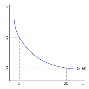
For simplicity, we will assume that a firm produces output using two types of inputs: labor and capital. All of the results that we will derive generalize in a straightforward manner when there are many inputs. The analysis of the multi-factor case, however, requires mathematical tools beyond the scope of this course. For now, we can think of labor as representing all of the inputs that are variable in the short run and capital as representing all of the inputs that are fixed in the short-run. Under this assumption, we can define as firm's short-run production function as: Q=f(L,K) where: Q = quantity of output produced The production function, f, is a mathematical function that provides the maximum quantity of output that can be produced for each possible combination of inputs used by the firm. A convenient way of representing this production function is through the use of a graph containing isoquant curves. An isoquant curve is a graph of all of the combinations of inputs that result in the production of a given level of output. (Note that the term "iso" means equal in Latin, thus the term "isoquant" literally means "equal quantity"). The diagram below contains a possible isoquant for a firm.
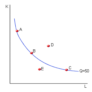
This isoquant suggests that the firm could produce 50 units of output per day using either 20 units of labor and 5 units of capital or 3 units of labor and 15 units of capital. In fact, any combination of labor and capital along this curve allows the firm to produce 50 units of output per day. Note that this curve is downward sloping because the firm can replace workers with machines or replace machines with workers and still manage to produce the same level of output. In the diagram below, the firm can produce 50 units of output using any of the input combinations given by points: A, B, or C. What happens, though, at point D? Is the firm producing more or less output at point D than at point C. When students are first asked this question, a common response is: "You cannot answer this since point D involves using more capital but less labor than is used at point C." But, what happens if we compare points B and D. At point D, the firm is using more labor and more capital than it is using at point B. If it uses more of each input it can produce more total output (assuming productive efficiency). Thus, we know that this firm can produce more output at point D than at point B. Since the firm produces 50 units of output at points A, B, and C, the output level corresponding to point B is higher than at any of the points on the isoquant. More generally, we can state that any point that lies above and to the right of an isoquant curve corresponds to a higher level of output. Using similar logic, the level of output will be lower if the firm selects a combination of inputs that lies below and to the left of an isoquant (as at point E in this diagram).
An isoquant curve passes through each and every point in this diagram. Two additional isoquant curves have been added to form the diagram below.
The isoquant curves considered above tell us about the physical ways in which inputs can be combined to produce output. Notice that they do not tell us anything about the costs associated with alternative levels of input use. (This topic will be considered below.)
|

