Form a sparse distributed representation of the input

When you imagine an input to a region, think of it as a large number of bits. In a brain these would be axons from neurons. At any point in time some of these input

bits will be active (value 1) and others will be inactive (value 0). The percentage of

input bits that are active vary, say from 0% to 60%. The first thing an HTM region does is to convert this input into a new representation that is sparse. For example, the input might have 40% of its bits “on” but the new representation has just 2% of its bits “on”.

 

An HTM region is logically comprised of a set of columns. Each column is comprised of one or more cells. Columns may be logically arranged in a 2D array but this is not a requirement. Each column in a region is connected to a unique subset of the input bits (usually overlapping with other columns but never exactly the same subset of

input bits). As a result, different input patterns result in different levels of activation of the columns. The columns with the strongest activation inhibit, or deactivate, the columns with weaker activation. (The inhibition occurs within a radius that can

span from very local to the entire region.) The sparse representation of the input is encoded by which columns are active and which are inactive after inhibition. The

inhibition function is defined to achieve a relatively constant percentage of columns to be active, even when the number of input bits that are active varies significantly.

 

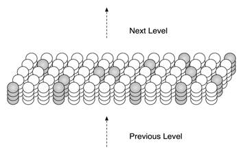
Figure 2.1: An HTM region consists of columns of cells. Only a small portion of a region is shown.

Each column of cells receives activation from a unique subset of the input. Columns with the strongest activation inhibit columns with weaker activation. The result is a sparse distributed representation of the input. The figure shows active columns in light grey. (When there is no prior state, every cell in the active columns will be active, as shown.)

 

Imagine now that the input pattern changes. If only a few input bits change, some columns will receive a few more or a few less inputs in the “on” state, but the set of active columns will not likely change much. Thus similar input patterns (ones that have a significant number of active bits in common) will map to a relatively stable set of active columns. How stable the encoding is depends greatly on what inputs

each column is connected to. These connections are learned via a method described later.

 

All these steps (learning the connections to each column from a subset of the inputs, determining the level of input to each column, and using inhibition to select a sparse set of active columns) is referred to as the “Spatial Pooler”. The term means

patterns that are “spatially” similar (meaning they share a large number of active bits) are “pooled” (meaning they are grouped together in a common representation).