GRAPHING AND VISUALIZATION IN MATHCAD
MathCAD provides a variety of two-dimensional X-Y and polar graphs plus three-dimensional contour, scatter, and surface plots.
1) Match useful words with the definitions:
2) Look through and remember the main elements of a graph:
Graphs are easy to create and modify in MathCAD. You can create 2D graphs from functions or data sets. A 2D graph can contain up to sixteen plots, all formatted differently.
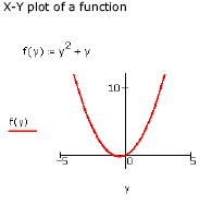
A. To create an X-Y Quick Plot of a single expression or function: 1. Type the expression or function of a single variable you want to plot. Click in the expression. 2. Choose Graph > X-Y Plot from the Insert menu. 3. Click outside the graph or press [Enter].
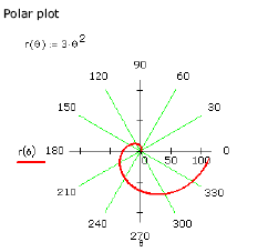
B. To create a polar plot: 1. Choose Graph > Polar Plot from the Insert menu. 2. Fill in both the angular-axis placeholder (bottom center) and the radial-axis placeholder (left center) with a function, expression, or variable. 3. Click outside the plot or press [Enter].
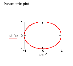
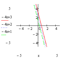
C. You can graph several traces on the same X-Y or polar plot. A graph can show several y-axis (or radial) expressions against the same x-axis (or angular) expression. Or it can match up several y-axis (or radial) expressions with the corresponding number of x-axis (or angular) expressions. To create a Quick Plot containing more than one trace: 1. Enter the expressions or functions of a single variable you want to plot, separated by commas. 2. Click in the expressions, then choose Graph > X-Y Plot from the Insert menu. 3. Click outside the graph or press [Enter].
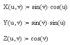
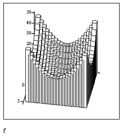
Three-dimensional plots enable you to visually represent a function of one or two variables and to plot data in the form of x-, y-, and z-coordinates.
A. To create a three-dimensional plot in MathCAD: 1. Define a function of two variables or a matrix of data. 2. Choose Grap h from the Insert menu and select a 3D plot type or click one of the 3D graph buttons on the Graph toolbar. 3. Enter the name of the function or matrix in the placeholder. 4. Click outside the plot or press [Enter] to see the plot.
B. The 3D Plot Wizard provides more control over the format settings of the plot as you insert it: 1. Choose Graph > Plot Wizard from the Insert menu. 2. Select a type of three-dimensional graph. 3. Make your selections for the appearance and coloring of the plot on subsequent pages of the Wizard. Click “Finish” and a graph region with a blank placeholder appears. 4. Enter appropriate arguments (a function name, data vectors, and so on) for the 3D plot into the placeholder. 5. Click outside the plot or press [Enter]. 1) Look at the graph and write the appropriate letters in front of each definition: 4. the horizontal axis (or the x axis) 5. a solid line 6. the vertical axis (or the y axis) 7. a broken line 8. the scale 9. a dotted line
http://www.eslflow.com/describinggraphstables.html
2) Use MathCAD to carry out the following tasks, comment your actions: A. Create a 3D Bar Plot of a function B. Give the plot a title “f(x,y)”, setting it below the graph. C. Convert the plot into a Surface plot. D. Draw light grey grid lines for all axes. E. Set x-axis limits with minimum value -6 and maximum value 6. F. Color the surface of the plot with light blue. G. Enable lighting on a 3D Plot, make a diffuse color light green and a specular color black. H. Set the axes at the front perimeter of the plot. I. Delete a rectangle around the graph. J. Draw a box around the plot. Make the border red.
|
 vertical axis/ y axis horizontal axis/ x axis
broken line dotted line
y-axis argument straight line
scale x-axis argument
curve
vertical axis/ y axis horizontal axis/ x axis
broken line dotted line
y-axis argument straight line
scale x-axis argument
curve

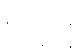 X-axis placeholder
Sizing grab-handle
X-axis placeholder
Sizing grab-handle


 y-axis scale placeholders
x-axis scale placeholders
3. To override MathCAD’s automatic limits by entering limits directly on the graph click a number in the scale placeholder, type a number to replace it and click outside the graph.
y-axis scale placeholders
x-axis scale placeholders
3. To override MathCAD’s automatic limits by entering limits directly on the graph click a number in the scale placeholder, type a number to replace it and click outside the graph.
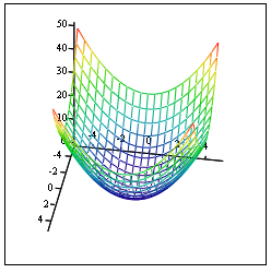
 Quick Plot from a function of two variables


 .
.