Simulation of an Inherently Discrete-Time System
We begin with an inherently discrete-time system most of us are familiar with, namely, a fixed interest loan with constant periodic payments. An amount of money is borrowed for a specified period of time, and equally spaced instalments are paid to the lender until the loan is completely repaid. The interest rate on the loan is established at the time of the loan. Furthermore, each payment consists of a portion that reduces the loan principal and the remaining portion that is interest on the outstanding balance. The situation is illustrated in Figure 3.1.
Fig. 3.1 Repayment and amortization of a loan.
The system parameters consist of:
The discrete-time input
is the constant payment A made at the end of the
The unpaid balance after the
It can be shown that the constant payment
Equations (3.5), (3.6), and (3.8) are the difference equations for the first-order discrete-time system in Figure 3.1.
Task A car loan in the amount of $125,000 is to be paid off in 30 years with an annual interest rate of 8%. Use the Simulink loan simulation to find (a) The monthly instalment (b) The unpaid balance after the 120th payment (c) The principal portion of the 200th payment (d) The total interest paid over the life of the loan (e) The time required for the unpaid balance to equal $62,500 Note the use of a single ‘‘Unit Delay’’ block to generate the signal Use Backward (implicit) Euler ‘‘Discrete–Time Integrator’’ for accurate computing. The ‘‘Simulation Parameters’’ dialog box is shown in Figure 3.2. A ‘‘Fixed–step’’ integrator with ‘‘Fixed-step size’’ of 1 is selected to force the simulation to step through integer values of discrete time. Since there is no continuous-time integration present in an inherently discrete-time system, the ‘‘discrete (no continuous states)’’ option is chosen from the drop-down menu of integrators.
Fig. 3.2 Simulation parameters dialog box for loan simulation.
The unpaid balance
Fig. 3.3 Unpaid balance The total monthly payment The total interest paid over the life of the loan is computed in two different ways. The simplest approach is to compute
Fig. 3.4 Monthly installment A Simulink diagram of the system is shown in Figure 3.5.
Fig. 3.5 Simulink diagram of loan repayment
Vocabulary:
|
 : Loan amount
 : Interest rate per period (fixed for the duration of the loan)
 : Number of interest periods for duration of loan
 th interest period. The discrete-time outputs are
 : Outstanding balance of loan immediately following the
  : Portion of
  : Interest portion of
  st payment is simply the unpaid balance following the

 , the portion of
  used for loan principal reduction, is equal to the reduction in outstanding balance from the
 , is obtained from
 necessary to fully repay the loan in
  , is given by
 as the difference of
  and the payment amount
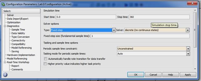
 .
.