Dominant firm model
In some markets there is a single firm that controls a dominant share of the market and a group of smaller firms. The dominant firm sets prices which are simply taken by the smaller firms in determining their profit maximizing levels of production. This type of market is practically a monopoly and an attached perfectly competitive market in which price is set by the dominant firm rather than the market. The demand curve for the dominant firm is determined by subtracting the supply curves of all the small firms from the industry demand curve.[7] After estimating its net demand curve (market demand less the supply curve of the small firms) the dominant firm maximizes profits by following the normal p-max rule of producing where marginal revenue equals marginal costs. The small firms maximize profits by acting as PC firms–equating price to marginal costs. Cournot-Nash model Main article: Cournot competition The Cournot-Nash model is the simplest oligopoly model. The models assumes that there are two “equally positioned firms”; the firms compete on the basis of quantity rather than price and each firm makes an “output decision assuming that the other firm’s behavior is fixed.”[8] The market demand curve is assumed to be linear and marginal costs are constant. To find the Cournot-Nash equilibrium one determines how each firm reacts to a change in the output of the other firm. The path to equilibrium is a series of actions and reactions. The pattern continues until a point is reached where neither firm desires “to change what it is doing, given how it believes the other firm will react to any change.”[9] The equilibrium is the intersection of the two firm’s reaction functions. The reaction function shows how one firm reacts to the quantity choice of the other firm.[10] For example, assume that the firm 1’s demand function is P = (60 - Q2) - Q1 where Q2 is the quantity produced by the other firm and Q1 is the amount produced by firm 1.[11] Assume that marginal cost is 12. Firm 1 wants to know its maximizing quantity and price. Firm 1 begins the process by following the profit maximization rule of equating marginal revenue to marginal costs. Firm 1’s total revenue function is PQ = Q1(60 - Q2 - Q1) = 60Q1- Q1Q2 - Q12. The marginal revenue function is MR = 60 - Q2 - 2Q.[12] MR = MC 60 - Q2 - 2Q = 12 2Q = 48 - Q2 Q1 = 24 - 0.5Q2 [1.1] Q2 = 24 - 0.5Q1 [1.2] Equation 1.1 is the reaction function for firm 1. Equation 1.2 is the reaction function for firm 2. To determine the Cournot-Nash equilibrium you can solve the equations simultaneously. The equilibrium quantities can also be determined graphically. The equilibrium solution would be at the intersection of the two reaction functions. Note that if you graph the functions the axes represent quantities.[13] The reaction functions are not necessarily symmetric.[14] The firms may face differing cost functions in which case the reaction functions would not be identical nor would the equilibrium quantities.
|


