The model of perfect competition.

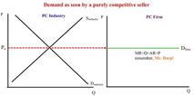
Demand as Seen by a Purely Competitive Seller:

Perfectly Elastic Demand:

Single Firm= small fraction of total output. Hence they are price-takers as they cannot influence market price. MANY firms TOGETHER can affect market price by changing industry output. Graphically perfectly elastic demand for single firm - horizontal line. ONLY ONE MARKET PRICE. Market demand for entire industry - downsloping curve. Firms can choose to produce at different market prices. If price changes at all it drastically affects quantity purchased i.e. price > equilibrium price causes quantity to go to zero and vice versa. A perfectly elastic demand means that the firm can produce as much as they want at that price and it will still be sold. Purchasers will be willing to buy any quantity at that price.

Average, Total, and Marginal Revenue:

Average Revenue (AR) schedule = demand schedule. Price per unit to buyer = revenue per unit to seller. Average revenue=price. Total Revenue (TR)= Price x Quantity (increases by constant amount – constant price). TR = P x Q. Straight upward sloping line – constant slope (= price). The area formed by the rectangle with coordinates (0,0), (0,P), (0,Q), (P,Q). Marginal Revenue (MR) = Change in Total Revenue from selling ONE additional unit of output. Same as price. MR = ∆ TR from selling 1 more unit of output = price. The reason MR=D=AR=P is because in a purely competitive firm the price carries over from the industry and thus that equals the demand. At this demand each additional output increases by the same degree and the average revenue at any point is the same price. Even with changes in the marketplace, the line may move vertically but the values will always be equal. Price line is the same as the average revenue or marginal revenue since the price is fixed.

Graphs: MR = AR = Demand = Price (represented by the horizontal line). This is because firms in a Purely Competitive Market are price-takers in that they MUST go with the industry equilibrium price (which is the intersection of S and D curve). См. график ниже:

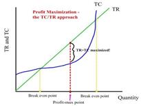
Profit Maximization in the Short-run: TR/TC Approach.

Firm = price taker → firms can only adjust output to maximize profit. Short-run = fixed plant → firms can only adjust amount of variable resource such as labor and materials.

Should we produce this product? Profit → Yes; Loss→ No. In what amount? Output level where economic profit is maximized TR– TC = (P x Q) - (FC + VC) = economic profits. Break-even point = when normal profit is satisfied. Intersection of TC + TR (TR covers all TC). No economic profit – only normal. There are 2 break-even points on graph – any point in between is economic profits. Profit is maximized on a graph where the vertical distance between TR and TC is the greatest.

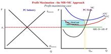
At break even point 1: the industry should PRODUCE MORE! At profit max point: the vertical distance between TR and TC is at its greatest, meaning the firm is earning maximum economic profits; therefore, industry should keep producing at this level of output, because more profits can still be made! At break even point 2: STOP PRODUCING! or REDUCE the quantity producing! TR and TC are equal, meaning the firm is now only earning a normal profit.

Profit Maximization in Short-run: MR/MC Approach.

Profit-maximizing case:

As long as MRDARP > AVC at the point where MC = MR, profit is maximized and production should continue. At any point where MR>MC, keep producing!! You can still profit more. At any point where MR<MC, reduce production. It only makes sense to produce less, because your costs are already more than what you're gaining. Firms must sell at the market price because

1) demand is perfectly elastic so higher price drops quantity consumed to zero

2) if price is decreased, ATC and AVC still remain unaffected, and economic profit decreases.

If Qpm = optimal outputs, then economic profit = Q(P-ATC)

Loss-minimizing case:

Even though the firm is not earning any economic profit, it is earning enough to pay their laborers (AVC), and thus it incurs less loss compared to the whole of average fixed cost.

In this situation, the company should continue producing the product. P = MR > AVC, P = MR < ATC --> point where MC = MR minimize its loss. Economic loss = Q (ATC - P). When AVC < P < ATC, the firm can stay open as long as they can cover the AVC. If a firm can cover all of the AVC and even part of the fixed costs, they will lose less than shutting down, as MR < ATC. Shutting down would mean losing everything and still have to pay for fixed costs, while in the loss minimizing case, costs are still covered.

Shut-down case:

This is when the amount of lost revenue that a firm gets from producing a unit is even greater than the cost of shutting down the company. (P = MR < AVC < ATC). The only time when a company should shut down! All the costs are above the equilibrium price line, meaning that the company will just lose money by producing its goods.