Simple regression analysis. The Simple Linear Model. Least Squares Regression. Interpretation of a Regression Equation.
Regression analysis – describes and evaluates the relationship between a given (dependent) variable and other independent variables. P – real economic data. X1 … four hypothetical values of the explanatory variables. If the relationship between Y and X were known the corresponding values of Y will be represented by the points Q1, Q2 … on the line. U - the disturbance term. U is positive in P1 and P4, and negative in P2 and P3. If you plot a line through the actual value of Y and X the line will cross P. The actual values of B1 and B2 and hence the location of the Q points are unknown as are the values of the U in the observations. The task of the regression analysis is to obtain estimates of B1 and B2 (slopes) and hence to estimate the location of the line given by P points. B1, B2 are the regression coefficients.
Why does U exist? 1) Omission of explanatory variables due to impossibility of obtaining them. 2)Aggregation of the variables. 3)Model misspecification. The model may be misspecified in terms of its structure. 4)Functional misspecification. The relationship between Y and X may be misspecified mathematically. 4)Measurement error. If the measurement of one or more variables in the relationship is wrong the relationship between Y and X will be wrong too. The equation of the fitted (regression) line is The caret mark over Calculating U. U is the difference between the actual and the estimated (fitted) value, and the distance between P1 and Q1. U is “e” .
simple linear regression fits a straight line through the set of P points in such a way that makes the sum of squared residuals of the model (that is, vertical distances between the P and the fitted line (Q)) as small as possible. We minimize RSS by using Ordinary Least Squares analysis.
We can influence the size of RSS only by changing B1 and B2, while Y and X are fixed. R2. For ex. R2=0.73 means that variance (дисперсия) of Y is described by this model on 73%. TSS=RSS+ESS
F-test (Fisher’s distribution)
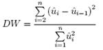
N number of observations (степени свободы, количество X), K-number of parameters (X, Y). It should be that F-test>Fcritic, means that the variance of “e” is equal. (дисперсия случайных величин, квадраты которых суммируются, одинакова.) and R2 is not random. Goodness of fit describes how well it fits a set of observations. Shows the discrepancy between observed values and the values expected under the model in question. Such measures can be used in statistical hypothesis testing, e.g. to test for normality of residuals, to test whether two samples are drawn from identical distributions 28.Ordinary Least Squares (OLS). The Gauss – Markov Theorem. Gauss-Markov theorem In Simple or Multiple Linear Regression, the model parameters are most often calculated by the Least Squares method. The main advantage of this method is its mathematical simplicity, which allows an easy identification of the statistical properties of the calculated estimators, in particular their bias (which is 0) and their covariance matrix. But there is no a priori reason to believe that these estimators are particularly good (low Mean Square Error of the parameters and of model predictions). The Gauss-Markov theorem is here to somewhat soften our worries about the quality of the Least Squares estimator of the vector of the model parameters. 1) E(Ui)=0 for all observations. Expected value of the disturbance term in any observation should be “0”. 2) σ_i^2=σ_2^2 Population variance of Ui constant for all observations. One of the tasks of the regression analysis is to estimate the standard deviation of the disturbance term. 3) Ui is distributed independently of Uj. It means that there should be no systematic association between the values of the disturbance term in any 2 observations. 4) U is distributed independently of the explanatory variables. The population covariance between the explanatory variable and the disturbance term is “0” 30.Heteroscedasticity. Possible Causes of Heteroscedasticity. The Goldfeld–Quandt Test. In statistics, sequence (последовательность) of random variables is heteroscedastic (H), if the random variables have different variances. In contrast, a sequence of random variables is called homoscedastic if it has constant variance. Heteroscedasticity does not cause ordinary least squares coefficient estimates (B1, B2) to be biased (смещенный), although it can cause ordinary least squares estimates of the variance (and, thus, standard errors) of the coefficients to be biased, possibly above or below the true or population variance. Thus, regression analysis using heteroscedastic data will still provide an unbiased estimate for the relationship between the predicted variable and the outcome, but standard errors and therefore conclusions obtained from data analysis may be biased. Biased standard errors lead to biased conclusions, so results of hypothesis tests are possibly wrong. Shortly, if H is present the OLS estimates are wrong, and the standard error of the regression coefficient will be wrong. Possible Causes of H. H is likely to be a problem when the values of the variables in the sample vary substantially in different observations. There may be a case that the variations in the omitted variables and the measurement errors that are responsible for the disturbance term will be relatively small when Y and X are small, and large when Y and X are large. The Goldfeld–Quandt Test is the most common test for H. If assume that the standard deviation of the probability distribution of the disturbance term in observation “i” is proportional to the size of If If we know standard deviation for each observation we can eliminate H by dividing each observation by its value of standard deviation. ANDREY?! 31.Autocorrelation. Possible Causes of Autocorrelation. The Durbin–Watson Test. Autocorrelation is a presence of series correlation between error terms. It describes a correlation between values of the process at different points in time, as a function of the two times or off the time difference. Positive autocorrelation, when on average if the residual (u) at time “t−1” is positive, the residual at time t is likely to be also positive; similarly, if the residual at t − 1 is negative, the residual at t is also likely to be negative. Negative autocorrelation, indicated by an alternating pattern in the residuals, when on average if the residual at time t − 1 is positive, the residual at time t is likely to be negative; similarly, if the residual at t − 1 is negative, the residual at t is likely to be positive. Autocorrelation is used in security analysis. For example, if you know a stock historically has a high positive autocorrelation value and you witnessed the stock making solid gains over the past several days, you might reasonably expect the movements over the upcoming several days (the leading time series) to match those of the lagging time series and to move upwards. In order to test for autocorrelation, it is necessary to investigate whether any relationships exist between the current value of the residuals and the previous values of the residuals. The most common diagnostic for presence of autocorrelation based on the estimated residuals
If there is positive autocorrelation in the errors, this difference in the numerator will be relatively small, while if there is negative autocorrelation, with the sign of the error changing very frequently, the numerator will be relatively large. The range of values between DW lies between 0 and 4. The closer it is to 0 then we get positive autocorrelation (cannot use OLS model). The closer it is to 4 we get negative autocorrelation (can use OLS model). The closer it is to 2 we get no autocorrelation. According to the 3d Gauss-Markov condition U should be distributed independently, so there should be no autocorrelation.
|
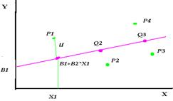
 =B1+B2*X1
 means that
  Substituting
  The e depends on the choice of B1 and B2 and should be close to zero. To solve this problem we should calculate RSS (residual Sum of Squares). If we can reduce RSS to zero we will have a perfect fit.


 в числителе находим среднее значение ошибки и делим ее на дисперсию.
 TSS(total sum of squares) is the sum, of the squares of the deviations (over all observations) of each observation from the overall mean;
 ESS (explained sum of squares) is the sum of the squares of the deviations of the predicted values from the mean value of a response variable.
 it is assumed that the disturbance term is normally distributed and satisfy other Gauss-Markov conditions.
 ,the model is HOMOscedsstic, and we CAN use OLS method, for all observations U is constant and satisfies 2d Gauss-Markov condition.
 is the Durbin and Watson test.